Pivot table with multiple, non hierarchical, columns

Question

Let's say my source data looks like this:

Brand   Model   Color   Region    Sales
---------------------------------------
Ford    Focus   Black   N/A       23
Ford    Focus   White   N/A       2
Nissan  Leaf    Black   N/A       12
Nissan  Leaf    White   N/A       6
Nissan  Pulsar  Black   N/A       3
Nissan  Pulsar  White   N/A       4
Ford    Focus   N/A     US        15
Ford    Focus   N/A     EU        10
Nissan  Leaf    N/A     US        5
Nissan  Leaf    N/A     EU        13
Nissan  Pulsar  N/A     US        1
Nissan  Pulsar  N/A     EU        6

I would like a pivot table that looked like this:

                   Color          Region
               Black   White     US    EU
------------------------------------------
Ford            
  Focus           23       2     15    10
Nissan
  Leaf            12       6      5    13
  Pulsar           3       4      1     6    

Is that possible? The only thing I can achieve is this:

                  Black         White            N/A
               US   EU   N/A  US  EU  N/A   US   EU   N/A
-----------------------------------------------------------
Ford            
  Focus                   23            2   15   10
Nissan
  Leaf                    12            6    5   13
  Pulsar                   3            4    1    6    

which is pretty ugly.

Problem seems to be that I'm not sure it's possible to have two variables in columns which are not hierarchically related. I could create two different pivot tables, onw wich brand/model/color and another with brand/model/region, but in my real case (that's a simple mockup) there're about 6-7 common variables, and having two huge tables is pretty overkill and not very pleasant for looking at data.

Thanks in advance for any help!

Answer 1

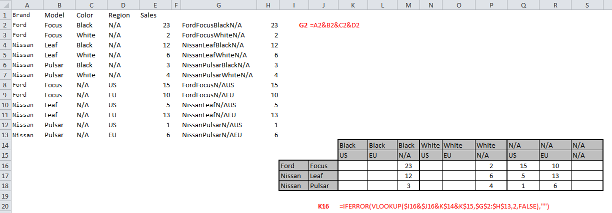
Solution below. It does look a bit too specific for what a pivot table can provide. I threw this together in 10min, so a more complicated one might take longer, but might be pretty difficult to maintain if your source changes a lot.

• I filled in Columns G and H, which are just a concatenation of your A-->D columns (G2= "=A2&B2&C2&D2"), and a copy of the total sales figure.
• Next I typed up the output table (what's in grey in I14--> S18)
• Then used the formula K16= "=IFERROR(VLOOKUP($I16&$J16&K$14&K$15,$G$2:$H$13,2,FALSE),"") " in K16 which pulls out the concatenation for the new table you want, and does a vlookup on our new table.
• You could clean it up a bit having use Black, White, N/A in the top row, and Nissan in the column only once, by changing the formula a bit. I did it this way so I could just dray and drop the cell.

Let me know if you want me to upload the excel file somewhere for you to look at.