Excel Pivot Table: Combining Data from Multiple Columns

Question

I'm trying to create a pivot table that summarizes Resource and Number of Days required per project phase. Each resource can appear across multiple phases for different durations. However, due to the amount of data that I have, I can't just add a phase column and then put a new row and line of data for each of the phases.

I can do this using countif and sumif, but due to the changing nature of my data and wanting to integrate slicers to cut the data with certain criteria, I need it to be in a pivot table.

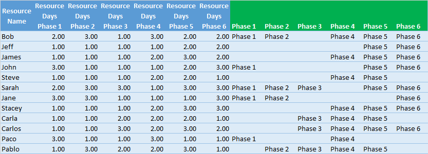
I do think the issue is likely how I have arranged this data; an example of which can be seen here:

The values are not just 1, 2, and 3 for the days in the real data set, but the purpose is that if Resource is over a certain value (not blank or 0) then this person works in that phase. My attempt to identify someone working in a particular phase were the phase columns, but they are not necessary as this was just my attempt at a solution.

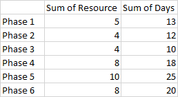
An example of how I am envisioning the output is below:

Answer 1

I do think the issue is likely how I have arranged this data

That is correct, to be able to use Pivot table in your data, your data structure should be like in the below screenshot.

In the above pivot table, the "count of days2" column is your "Sum of Resources"

Please find the Sample Excel at the following link:
https://drive.google.com/open?id=1Szayirw84TXll8y6ASvZBtlxKrkN3nK5

Answer 2

This would be easier if you were starting from a layout that was designed for summarizing, but you can actually do it in a few simple steps. I recreated just the first few relevant data columns

The first step is adding the resource and days totals at the end of each column. The Resources total in H14 is:

=COUNTA(H2:H13)

This just counts cells with an entry in the column. The Days total in H15 is:

=SUMIF(H2:H13,H$1,B2:B13)

This sums the values in the associated column B if column H contains a value that matches the column header. If your actual spreadsheet is different, just use a relevant test condition, which could be simply "not blank".

Once you've entered the first two formulas, you can copy or drag them across to fill the other columns.

To get the results in columns O through Q, select the header range with the column labels, then hold the Ctrl key to select and add the formulas since it isn't all contiguous. Copy the selection (Ctrl+C or the Copy icon in the toolbar).

I manually added the column headings in P and Q. To fill in the values, click into the upper left corner of where the results will go (O2 in this case), right-click and select Paste Special. Select Values and Transpose and click OK.