1

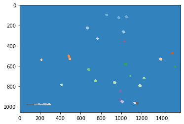
I have the following image.image I was able to use watershed to detect all the particles using the code below.

However, now I need to calculate the size of each particles in the figure and if I use the "labels" image, for some reasons I am not capable of using the function cv2.findContours.

Anyone willing to share some ideas? If you propose some code, please include explanation because I am a beginner. :)

Many thanks!

import numpy as np
import cv2
import matplotlib.pyplot as plt
from scipy import ndimage as ndi
from skimage.morphology import watershed
from skimage.feature import peak_local_max

#-------------------------------------------------------------------------------------------#
# IMAGE PRETREATMENT

img = cv2.imread('Test images/TEM of nanoparticles/NP good 0010.tif')
gray = cv2.cvtColor(img,cv2.COLOR_BGR2GRAY)


Gaussian_Blur = cv2.GaussianBlur(gray,(21, 21), cv2.BORDER_DEFAULT)

# Use fixed threshold to mask black areas
_, thresh = cv2.threshold(Gaussian_Blur, 90, 255, cv2.THRESH_BINARY_INV) # _ = 30

# Morphological closing to close holes inside particles; opening to get rid of noise
img_mop1 = cv2.morphologyEx(thresh, cv2.MORPH_CLOSE, cv2.getStructuringElement(cv2.MORPH_ELLIPSE, (7, 7)))
img_mop = cv2.morphologyEx(img_mop1, cv2.MORPH_OPEN, cv2.getStructuringElement(cv2.MORPH_ELLIPSE, (15, 15)))
tiled_h = np.hstack((img_mop1, img_mop)) # stack images side-by-side

plt.figure('Pretreatment')
plt.subplot(2, 2, 1) # Figure two has subplots 2 raw, 2 columns, and this is plot 1
plt.gca().set_title('Gray')
plt.xticks([]), plt.yticks([]) # To hide axes
plt.imshow(gray, cmap='gray')

plt.subplot(2, 2, 2) # Figure two has subplots 2 raw, 2 columns, and this is plot 1
plt.gca().set_title('Gaussian_Blur')
plt.xticks([]), plt.yticks([]) # To hide axes
plt.imshow(Gaussian_Blur, cmap='gray')

plt.subplot(2, 2, 3) # Figure two has subplots 2 raw, 2 columns, and this is plot 1
plt.gca().set_title('Thresh')
plt.xticks([]), plt.yticks([]) # To hide axes
plt.imshow(thresh, cmap='gray')

plt.subplot(2, 2, 4) # Figure two has subplots 2 raw, 2 columns, and this is plot 1
plt.gca().set_title('img_mop')
plt.xticks([]), plt.yticks([]) # To hide axes
plt.imshow(img_mop, cmap='gray')


#-------------------------------------------------------------------------------------------#
# WTERSHED WITH SKIMAGE

# Now we want to separate the two objects in image
# Generate the markers as local maxima of the distance to the background
distance = ndi.distance_transform_edt(img_mop) # Calculates distance of pixels from background

#Find peaks in an image as coordinate list or boolean mask.
local_maxi = peak_local_max(distance, indices=False, footprint=np.ones((3, 3)), labels=img_mop)
# indices: if True, the output will be an array representing peak coordinates. If False, the output will be a boolean
# array shaped as image.shape with peaks present at True elements.
# If footprint == 1 represents the local region within which to search for peaks at every point in image.
# labels: if provided, each unique region labels == value represents a unique region to search for peaks. Zero is
# reserved for background.
# returns an array of boolean with True on max points
print('local_maxi lenght: ', local_maxi.shape)
print('local_maxi: ', local_maxi[0])
markers = ndi.label(local_maxi)[0]
print('markers lenght: ', markers.shape)
print('markers: ', markers[0])
labels = watershed(-distance, markers, mask=img_mop)
print('labels lenght: ', labels.shape)
print('labels: ', labels[0])


plt.figure('Processing')
plt.subplot(2, 2, 1) # Figure two has subplots 2 raw, 2 columns, and this is plot 1
plt.gca().set_title('Distance trans')
plt.xticks([]), plt.yticks([]) # To hide axes
plt.imshow(distance, cmap='gray')

plt.subplot(2, 2, 2) # Figure two has subplots 2 raw, 2 columns, and this is plot 1
plt.gca().set_title('local_maxi')
plt.xticks([]), plt.yticks([]) # To hide axes
plt.imshow(local_maxi, cmap='gray')

plt.subplot(2, 2, 3) # Figure two has subplots 2 raw, 2 columns, and this is plot 1
plt.gca().set_title('markers')
plt.xticks([]), plt.yticks([]) # To hide axes
plt.imshow(markers, cmap='gray')

plt.figure('Watershed')
plt.gca().set_title('Watershed')
plt.xticks([]), plt.yticks([]) # To hide axes
plt.imshow(labels, cmap='gray')

plt.show()

#-------------------------------------------------------------------------------------------#
# DATA ANALYSIS ---- WORK IN PROGRESS

cnts, _ = cv2.findContours(labels, cv2.RETR_EXTERNAL, cv2.CHAIN_APPROX_NONE)
img = cv2.drawContours(img, cnts, -1, (0, 255, 255), 2) # To print all contours
cv2.imshow('Contours',  cv2.resize(img, dsize=(0, 0), fx=0.3, fy=0.3))
print('\nCnts length: ', len(cnts), '\n') # 11 objects (10 nanoparticles + scale barr)


# Divide the cnts array into scalebar and nanoparticles
# Get bounding rectangles for the scale and the particles from detailed contour determine on line 32.
# cv2.boundingRect() outputs: x, y of starting point (top left corner), and width and height of rectangle.
# Find contours. For more info see: https://opencv-python-tutroals.readthedocs.io/en/latest/py_tutorials/py_imgproc/py_contours/py_contour_features/py_contour_features.html
# cv2.contourArea() outputs the area of each detailed contour, does not work on rectangle generated by cv2.boundingRect.
thr_size = 5000
for cnt in cnts:
    if cv2.contourArea(cnt) > thr_size:
        scale = [cv2.boundingRect(cnt)] # returns x, y, w, h

img = cv2.rectangle(img, (scale[0][0], scale[0][1]), (scale[0][0] + scale[0][2], scale[0][1] + scale[0][3]), (255, 255, 0), 2)
print('Scale is: ', scale) #only one box (object) = scalebar
print("scale[0][1] is scalebar's width of {} pixels".format(scale[0][2]), '\n')


# 8. MINIMUM ENCLOSING CIRCLE
i = 1
for cnt in cnts:
    if cv2.contourArea(cnt) < thr_size:
        # Find min enclosing circle and get xy of centre
        (x, y), radius = cv2.minEnclosingCircle(cnt)
        center = (int(x), int(y))

        # Get radius average method
        #rx, ry, w, h = cv2.boundingRect(cnt)
        #radius = int((((w+h)/2))*1.5)
        img = cv2.circle(img, center, radius, (255, 0, 255), 3)

        cv2.putText(img, str(i), (int(x), int(y)-20), cv2.FONT_HERSHEY_COMPLEX, 1, (0, 255, 0), 2)
        print('Particle ' + str(i) + ' | Horizontal diameter: ' + '{:.2f}'.format((radius/ scale[0][2] * 200)*2) + ' nm')
        i=i+1
cv2.imshow('img',  cv2.resize(img, dsize=(0, 0), fx=0.3, fy=0.3))
0

3 Answers 3

3

I am sharing an approach with watershed and regionprops

from skimage import io
import numpy as np
import matplotlib.pyplot as plt
from skimage.feature import peak_local_max
from skimage.measure import regionprops
from skimage.morphology import watershed
from scipy.ndimage.morphology import binary_erosion, binary_dilation, distance_transform_edt
from scipy.ndimage import label

import pandas as pd


img = io.imread('obvvX.jpg')

a = gaussian(img, sigma=5)
a = np.sum(a, axis=2)
a_thr = a < 1
plt.imshow(a)

# clean up specks
a_thr = binary_erosion(a_thr, iterations = 5)
a_thr = binary_dilation(a_thr, iterations = 5)

# do distance transform as prepartion for watershed
distances = distance_transform_edt(a_thr)

# find watershed seeds
seeds = peak_local_max(distances, indices =False, min_distance=20, footprint=np.ones((3,3)))
seeds = label(seeds)[0]

# watershed
ws = watershed(a, seeds, mask=a_thr)

plt.imshow(ws, cmap='tab20c')

enter image description here

So, the scale bar is also recognised as objects. We can now use regionprops to get the areas:

# compute region properties
props = regionprops(ws)

# exclude the bar on the bottom left:
props = [p for p in props if p['centroid'][0]<950 and p['centroid'][1]>400]

# get the sizes for each of the remaining objects and store in dataframe
entries = []
for p in props:
    entry = [p['label'], p['area'], p['perimeter'], *p['centroid']]
    entries.append(entry)


df = pd.DataFrame(entries, columns= ['label', 'area', 'perimeter', 'y', 'x'])

The dataframe has some entries that are too small to be actual objects. These can be deleted by setting a lower size threshold:

df = df[df['area'] > 40]


label  area perimeter   y           x
0   1   432 75.012193   17.048611   1182.236111
1   2   490 79.254834   48.781633   679.438776
2   3   580 86.083261   98.012069   851.260345
3   4   601 89.740115   116.382696  1047.943428
4   5   729 98.911688   126.149520  972.554184
5   6   595 88.669048   226.092437  663.673950
6   7   664 94.325902   263.808735  1018.560241
7   8   136 43.313708   323.875000  756.867647
8   9   382 107.012193  332.437173  764.958115
11  12  69  36.041631   359.420290  1028.507246
12  13  386 70.426407   475.414508  1498.546632
14  15  576 117.876154  503.248264  481.036458
18  19  146 60.656854   524.890411  484.308219
19  20  415 89.597980   532.655422  492.667470
20  21  580 114.118795  533.408621  1383.151724
22  24  695 96.568542   581.585612  1038.273381
23  25  288 71.976659   605.114583  1522.270833
24  26  77  32.485281   611.610390  1529.779221
26  28  666 124.704581  634.734234  676.509009
27  29  205 52.769553   696.921951  1083.165854
28  30  555 84.426407   719.812613  1220.690090
29  31  605 88.669048   745.538843  743.304132
31  33  637 119.497475  762.742543  931.612245
32  34  491 79.254834   784.340122  410.175153
33  35  700 97.154329   793.735714  1179.764286
34  36  712 96.911688   846.039326  987.450843
35  37  528 89.740115   932.549242  984.071970
2
  • Thanks warped! The solution is on the use of regionprops! For people interested in learning more, see: # scikit-image.org/docs/dev/api/…
    – Pier
    Commented Dec 15, 2019 at 13:19
  • 1
    Also, @warped, we now have regionprops_table as a convenient way to create that for-loop! =) Thanks for the thorough response!
    – Juan
    Commented Dec 16, 2019 at 11:06
1

Here is one way to do it using blobs in Python/OpenCV.

  • Read the image
  • Convert to grayscale
  • Gaussian smooth the image to reduce noise
  • Apply adaptive thresholding
  • Use Simple Blob Detector with appropriate limits on characteristics to get key points and their size and locations

Input:

enter image description here

import numpy as np
import cv2
import math

# read image
img = cv2.imread("particles.jpg")

# convert to grayscale
gray=cv2.cvtColor(img,cv2.COLOR_BGR2GRAY)

# apply Gaussian Blur
smoothed = cv2.GaussianBlur(gray, (0,0), sigmaX=9, sigmaY=9, borderType = cv2.BORDER_DEFAULT)

# do adaptive threshold on gray image
thresh = cv2.adaptiveThreshold(smoothed, 255, cv2.ADAPTIVE_THRESH_MEAN_C, cv2.THRESH_BINARY, 65, 10)

cv2.imshow("Threshold", thresh)
cv2.waitKey(0)
cv2.destroyAllWindows()

# Set up the SimpleBlobdetector with default parameters.
params = cv2.SimpleBlobDetector_Params()

# Change thresholds
params.minThreshold = 0
params.maxThreshold = 256

# Filter by Area.
params.filterByArea = True
params.minArea = 30
params.maxArea = 10000

# Filter by Color (black=0)
params.filterByColor = True
params.blobColor = 0

# Filter by Circularity
params.filterByCircularity = True
params.minCircularity = 0.5
params.maxCircularity = 1

# Filter by Convexity
params.filterByConvexity = True
params.minConvexity = 0.5
params.maxConvexity = 1

# Filter by InertiaRatio
params.filterByInertia = True
params.minInertiaRatio = 0
params.maxInertiaRatio = 1

# Distance Between Blobs
params.minDistBetweenBlobs = 0

# Do detecting
detector = cv2.SimpleBlobDetector_create(params)

# Get keypoints
keypoints = detector.detect(thresh)

print(len(keypoints))
print('')

# Get keypoint locations and radius
for keypoint in keypoints:
   x = int(keypoint.pt[0])
   y = int(keypoint.pt[1])
   s = keypoint.size
   r = int(math.floor(s/2))
   print (x,y,r)
   #cv2.circle(img, (x, y), r, (0, 0, 255), 2)

# Draw blobs
blobs = cv2.drawKeypoints(thresh, keypoints, np.array([]), (0,0,255), cv2.DRAW_MATCHES_FLAGS_DRAW_RICH_KEYPOINTS)
cv2.imshow("Keypoints", blobs)
cv2.waitKey(0)
cv2.destroyAllWindows()

# Save result
cv2.imwrite("particle_blobs.jpg", blobs)


Results:

25 points:

1143 965 19
996 942 22
131 928 9
158 920 5
85 921 7
987 845 15
1180 794 15
411 784 15
932 762 14
743 745 14
1221 719 13
677 635 15
1523 606 14
1039 581 14
211 539 15
1383 533 14
486 516 21
1498 474 13
763 330 13
1019 264 14
664 226 14
973 126 15
1048 116 14
852 99 14
679 49 14


Output Image:

enter image description here

See this example for discussion of arguments

A second approach might be to get the contours in place of the blobs. Then get the bounding boxes of the contours and from that compute the radii and centers.

A third approach might be to use connected components with stats. Again it would get the bounding boxes and areas and centroids from which you could compute the radius and draw circles.

2
  • Thanks for your answer, very much appreciated! I have done the same for a similar image, but what I am trying to do now is to use watershed segmentation to separate those 2-3 groups of 2 attached nanoparticles and calculate their size. As you can see your code for those cases gives an enclosing circle that is much larger because consider both particles together. I could potentially just divide the area by 2, but I was hoping that with watershed I could be more precise.
    – Pier
    Commented Dec 15, 2019 at 13:15
  • Sorry, I misunderstood your question.
    – fmw42
    Commented Dec 15, 2019 at 19:18
1

By following the example of warped, I was able to pretty much solve the problem. You can find the new code below. I though that this might be useful to others.

I still have some questions though: 1) Watershed segmentation finds more areas than expected. For example, if you closely check one of those binary clusters of nanoparticles, it finds 3-4 different areas instead of just 2. These areas are usually small and I got rid of them using a size threshold, as warped suggested. However, is it possible to fine tune the watershed to somehow merge those areas and get a more accurate result?

2) I prefer using cv2.imshow() to show the images. However for some reasons I cannot plot the watershed result (variable name: labels) with that command, that's why I used matplotlib in the first part of the code. Does anyone have an explanation and a fix for this?

import numpy as np
import cv2
import matplotlib.pyplot as plt
from scipy import ndimage as ndi
from skimage.morphology import watershed
from skimage.feature import peak_local_max
from skimage.measure import regionprops

#----------------------------------------------------------------------------------------------------------------------#
# IMAGE PRETREATMENT

img = cv2.imread('Test images/TEM of nanoparticles/NP good 0010.tif')
gray = cv2.cvtColor(img,cv2.COLOR_BGR2GRAY)
Gaussian_Blur = cv2.GaussianBlur(gray,(21, 21), cv2.BORDER_DEFAULT)

# Use fixed threshold to mask black areas
_, thresh = cv2.threshold(Gaussian_Blur, 90, 255, cv2.THRESH_BINARY_INV) # _ = 30

# Morphological closing to close holes inside particles; opening to get rid of noise
img_mop1 = cv2.morphologyEx(thresh, cv2.MORPH_CLOSE, cv2.getStructuringElement(cv2.MORPH_ELLIPSE, (7, 7)))
img_mop = cv2.morphologyEx(img_mop1, cv2.MORPH_OPEN, cv2.getStructuringElement(cv2.MORPH_ELLIPSE, (15, 15)))
tiled_h = np.hstack((img_mop1, img_mop)) # stack images side-by-side

plt.figure('Pretreatment')
plt.subplot(2, 2, 1) # Figure two has subplots 2 raw, 2 columns, and this is plot 1
plt.gca().set_title('Gray')
plt.xticks([]), plt.yticks([]) # To hide axes
plt.imshow(gray, cmap='gray')

plt.subplot(2, 2, 2)
plt.gca().set_title('Gaussian_Blur')
plt.xticks([]), plt.yticks([])
plt.imshow(Gaussian_Blur, cmap='gray')

plt.subplot(2, 2, 3)
plt.gca().set_title('Thresh')
plt.xticks([]), plt.yticks([])
plt.imshow(thresh, cmap='gray')

plt.subplot(2, 2, 4)
plt.gca().set_title('img_mop')
plt.xticks([]), plt.yticks([])
plt.imshow(img_mop, cmap='gray')


#----------------------------------------------------------------------------------------------------------------------#
# WTERSHED WITH SKIMAGE

distance = ndi.distance_transform_edt(img_mop) # Calculates distance of pixels from background

#Find peaks in an image as coordinate list or boolean mask.
local_maxi = peak_local_max(distance, indices=False, min_distance=50, footprint=np.ones((3, 3)), labels=img_mop)
markers = ndi.label(local_maxi)[0]
labels = watershed(-distance, markers, mask=img_mop)

plt.figure('Processing')
plt.subplot(2, 2, 1) # Figure two has subplots 2 raw, 2 columns, and this is plot 1
plt.gca().set_title('Distance trans')
plt.xticks([]), plt.yticks([]) # To hide axes
plt.imshow(distance, cmap='gray')

plt.subplot(2, 2, 2)
plt.gca().set_title('local_maxi')
plt.xticks([]), plt.yticks([])
plt.imshow(local_maxi, cmap='gray')

plt.subplot(2, 2, 3)
plt.gca().set_title('markers')
plt.xticks([]), plt.yticks([])
plt.imshow(markers, cmap='gray')

plt.figure('Watershed')
plt.gca().set_title('Watershed')
plt.xticks([]), plt.yticks([]) # To hide axes
plt.imshow(labels)

plt.show()

#----------------------------------------------------------------------------------------------------------------------#
# DATA ANALYSIS

# Regionprops: Measure properties of labeled image regions. It can give A LOT of properties, see info in:
# https://scikit-image.org/docs/dev/api/skimage.measure.html#skimage.measure.regionprops
props = regionprops(labels)

# Determine scale bar (largest object) and set the scale.
thr_size = 6000
for p in props:
    if p['area'] > thr_size:
        box = p['bbox']
        scale = box[3]-box[1]


# Remove smaller detected areas, and give area and diameter for each of the remaining particles.
for p in props:
    if p['equivalent_diameter'] > 15 and p['equivalent_diameter'] < 40:
        entry = [p['label'], p['area'], p['equivalent_diameter'], *p['centroid']]
        n = entry[0]
        y = entry[3]
        x = entry[4]-60 # so that number shows on the left of particle
        cv2.putText(img, str(n), (int(x), int(y)), cv2.FONT_HERSHEY_COMPLEX, 1, (0, 255, 0), 2)
        print('Particle {} | Area (nm^2): {}; Equivalent diameter (nm): {}'.format(str(n),
                                            str(int(((entry[1]*40000)/(scale**2)))), str(int((entry[2])*200/scale))))

cv2.imshow('img', img)
cv2.waitKey(0)
cv2.destroyAllWindows()

Your Answer

By clicking “Post Your Answer”, you agree to our terms of service and acknowledge you have read our privacy policy.

Not the answer you're looking for? Browse other questions tagged or ask your own question.