suspension system

Asad Asghar Janjua

suspension system

Asad Asghar Janjua

visibility

…

description

9 pages

link

1 file

Captivate. Motivate. graduate. Quanser educational solutions are powered by:  

Figures (6)

“Please note: The Hexapod is not available for purchase in North America, Japan and Taiwan. Full range of robotic and mechatronic control plants for teaching and research

laboratory guide active Suspension experiment for Matlab /Simulink users Developed by: Jacob Apkarian, Ph.D., Quanser Amin Abdossalami, M.A.SC., Quanser Quanser educational solutions are powered by: Captivate. Motivate. graduate. PREFACE Preparing laboratory experiments can be time-consuming. Quanser understands time constraints of teaching and resear h professors. That’s why Quanser’s ontrol la oratory solutions come with proven practical exercises. The courseware is designed to save you time, give students a solid understanding of various control concepts and provide maximum value for your investment. Quanser Active Suspension courseware materials are supplied in a format of the Laboratory Guide. The Lab Guide contains lab assignments for students. This course material is prepared for users of The MathWorks’s MATLAB/Simulink software in conjunction with Quanser’s QUARC real-time control software. A version of the course material for National Instruments LabVIEW™ users is also available. The following material provides an abbreviated example of in-lab procedures for the Active Suspension experiment. Please note that the examples are not complete as they are intended to give you a brief overview of the structure and content of the courseware materials you will receive with the plant.   TABLE OF CONTENTS PREFACE ...................................................................................................................... PAGE 1 INTRODUCTION TO QUANSER ACTIVE SUSPENSION COURSEWARE SAMPLE .......... PAGE 3 LABORATORY GUIDE TABLE OF CONTENTS ................................................................ PAGE 4 BACKGROUND SECTION – SAMPLE ............................................................................ PAGE 5 LAB EXPERIMENTS SECTION – SAMPLE ...................................................................... PAGE 6   1. INTRODUCTION TO QUANSER ACTIVE SUSPENSION COURSEWARE SAMPLE Quanser courseware materials provide step-by-step pedagogy for a wide range of control challenges. Starting with the basic principles, students can progress to more advanced applications and cultivate a deep understanding of control theories. Quanser 2 DOF Inverted Pendulum courseware covers topics, such as:  How to mathematically model the Active Suspension plant, using, for example, force analysis on free body diagrams  How to obtain a state-space representation of the open-loop system and to do open-loop analysis  How to obtain different transfer functions for the Active Suspension Experiment as a MIMO system  How to use the obtained Active Suspension state-space representation to design a Linear Quadratic Regulator (LQR)  To simulate the Linear Quadratic Estimator/Regulator (LQE/LQR) controller using the developed model of the plant and to ensure the controller performance specifications are met without any actuator saturation  To implement an LQR-based state-feedback controller in real-time and evaluate its actual performance  To observe and investigate the disturbance response of the suspension system in response to chirp and pulse shape road disturbances   2. LABORATORY GUIDE TABLE OF CONTENTS The full Table of Contents of the Quanser Active Suspension Laboratory Guide is shown here: 1. INTRODUCTION 1.1. DESCRIPTION 1.2. TOPICS COVERED 2. BACKGROUND 2.1. MODELING 2.1.1. DYNAMICS 2.1.2. ELIMINATING GRAVITY FORCE FROM EOM 2.1.3. STATE-SPACE REPRESENTATION 2.1.4. SYSTEM TRANSFER FUNCTIONS 2.2. CONTROL 2.2.1. STABILITY 2.2.2. CONTROLLABILITY 2.2.3. LINEAR QUADRATIC REGULATOR (LQR) 3. IN-LAB PROCEDURES 3.1. SIMULATION 3.1.1. PROCEDURE 3.1.2. ANALYSIS 3.2. IMPLEMENTATION 3.2.1. CLOSED-LOOP CONTROL 3.2.2. OPEN-LOOP ANALYSIS 4. SYSTEM REQUIREMENTS 4.1. OVERVIEW OF FILES 4.2. SETUP FOR SIMULATION 4.3. SETUP FOR EXPERIMENT REFERENCES   3. BACKGROUND SECTION - SAMPLE Modeling - Dynamics In this section, the general dynamic equations of the Active Suspension System will be derived. The Free Body Diagram method is used to obtain the dynamics of the system as a double mass-spring damper model. This diagram is illustrated in Figure 2.1. In this approach, the two inputs to the system are considered to be active suspension control command Fc and the road surface position zr. Furthermore, it is reminded that the reference frames in Figure 2.1 are used to choose the generalized coordinates, i.e. x1 and x2. The generalized coordinate x1 represents the tire displacement (usnprung mass in quarter car model) and x2 represents the vehicle body displacement (sprung mass in the quarter car model) all with respect to the ground. The positive directions are upwards. Figure 2.1: Double Mass-Spring-Damper used to model Active Suspension Experiment To find out equations of motion (EOM) for this system, the free body diagram for each mass should be determined. There are two masses in the system and the forces applied to each mass should be drawn on the diagrams. There will be two equations of motion. All the initial conditions are assumed to be zero. The free body diagram for Ms looks like Figure 2.2. The forces applied to the Ms are due to the spring force, damping force, active suspension force, and gravity. Figure 2.2: The free body diagram for Ms The EOM for Ms will be as follows (2.1)   4. LAB EXPERIMENTS SECTION - SAMPLE Simulation The state space representation of Active Suspension was derived in Equation 2.11. In this section, you will generate those equations and design a controller. The parameter values are outlined in the table below. These values have been derived using system identification techniques and they might not exactly match the nominal values presented in the ASE User Manual. Parameter Symbol Parameter Name Parameter Value Ms Sprung Mass 2.45 kg Mus Unsprung Mass 1 kg Ks Suspension Stiffness 900 N/m Kus Tire Stiffness 1250 N/m Bs Suspension Inherent Damping Coefficient 7.5 Nsec/m Bus Tire Inherent Damping Coefficient 5 Nsec/m Table 3.1: Active Suspension Experiment Parameter Nomenclature. In this section we will use the Simulink diagram shown in Figure 3.1 to simulate the closed-loop control of the Active Suspension system. The system is simulated using the model summarized in Section 2.1. The Simulink model uses state-feedback control, with feedback gain K found using the Matlab LQR command (LQR is described briefly in Section 2.2.3). Figure 3.1: Simulink model used to simulate Active Suspension. IMPORTANT: Before you can conduct these simulations and experiments, you need to make sure that the lab files are configured according to your setup. If they have not been configured already, then you need to go to Section 4 to configure the lab files first. Procedure Follow these steps to simulate the system: 1. Make sure the LQR weighting matrices in setup_as.m are set to And R = 0.01 2. Run the script to generate the gain K = [24.66 48.87 -0.47 3.68]. 3. Open the plate position scope, Simulation zr_zs_zus. 4. The road input is a square shape signal with an amplitude of 0.01 m and frequency of 0.3Hz   4. 5. Zr represents the bottom plate position which refers to the road. Zus represents the middle plate position which refers to vehicle tire. Zs represents the top plate position which refers to vehicle body. 6. In the Simulink diagram, go to QUARC  Build. 7. Click Connect to Target to connect to the real-time code, then Click on QUARC  Start to run simulation. 8. The active damping control action can be enabled or disabled using the Manual Switch to observe both the controller performance and open loop response. 9. The scopes should be displaying a response similar to Figure 3.2. The closed loop controller is enabled 5 seconds into the response. Figure 3.2: Simulated closed-loop response. Analysis In the closed loop system the vehicle body and tire exhibit smaller oscillations in response to the road disturbances. The acceleration signal amplitude is also smaller in closed loop which indicates a better comfort measure in the quarter-car system. The tire oscillations are also dampened which indicates a better road handling measure. 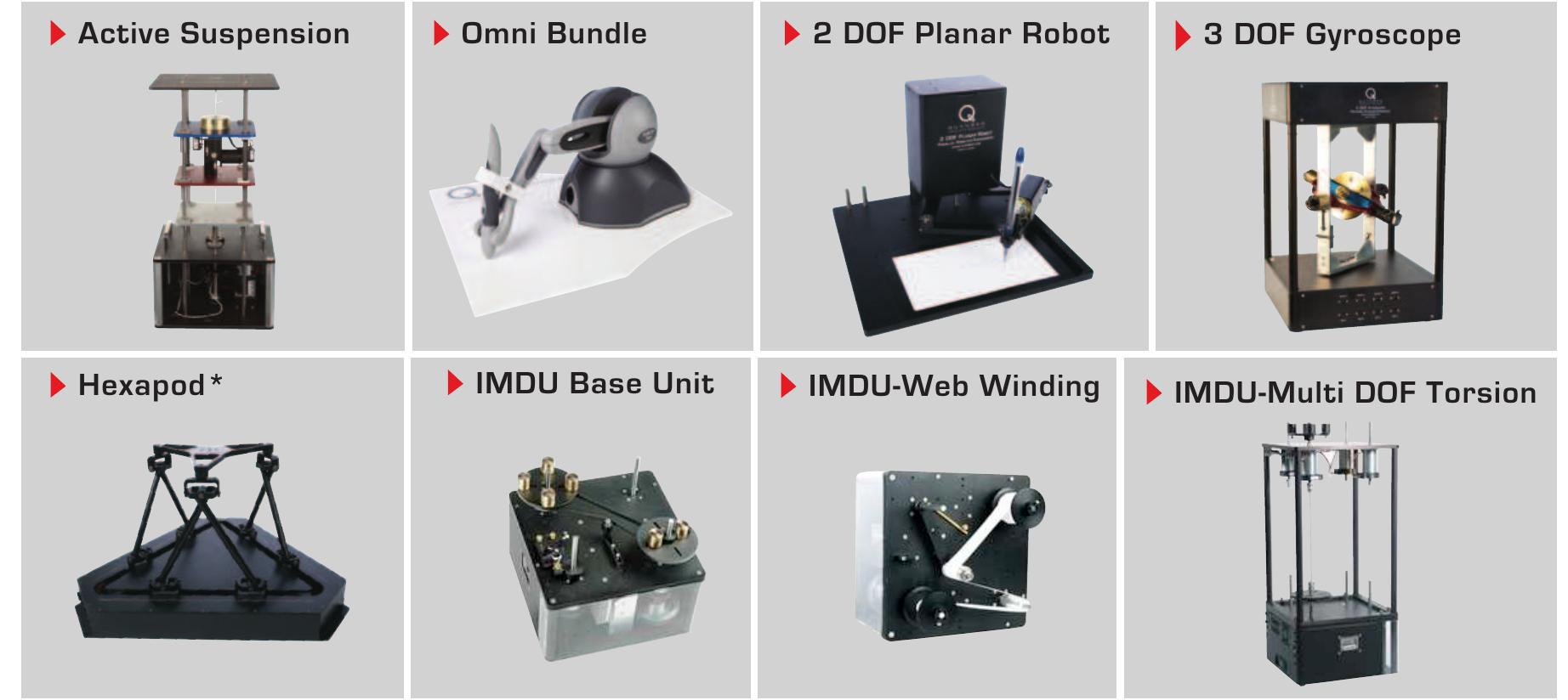  Full range of robotic and mechatronic control plants for teaching and research active Suspension Hexapod* omni bundle iMdu base unit 2 doF planar robot iMdu-Web Winding 3 doF gyroscope iMdu-Multi doF torsion * Please note: The Hexapod is not available for purchase in North America, Japan and Taiwan. Choose from eight plants to create experiments for teaching or research related to robotics, haptics, mechatronics, aerospace, or process control. For more information please contact [email protected] ©2013 Quanser Inc. All rights reserved. [email protected] +1-905-940-3575 Solutions for teaching and research. Made in Canada. QuaNSer.CoM

Log In

suspension system

Sign up for access to the world's latest research

Figures (6)

Related papers

Related papers

Related topics