STUDY & VIBRATION ANALYSIS OF GRADUAL DECREASE BEAM BY FEM

International Journal of Mechanical Engineering and Technology (IJMET) Volume 9, Issue 1, January 2018, pp. 431–444, Article ID: IJMET_09_01_047 Available online at http://www.iaeme.com/IJMET/issues.asp?JType=IJMET&VType=9&IType=1 ISSN Print: 0976-6340 and ISSN Online: 0976-6359 © IAEME Publication Scopus Indexed STUDY & VIBRATION ANALYSIS OF GRADUAL DECREASE BEAM BY FEM Mani Kant M.Tech. Scholar, Dept. of Mechanical Engineering, SHUATS, Allahabad, U.P., India Dr. Prabhat Kumar Sinha Assistant Professor, Department of Mechanical Engineering, SHUATS Allahabad, U.P., India ABSTRACT In this study the important member beam are used as structural components and it can be classified according to their geometric configuration as uniform or taper and slender or thick. If practically analyzed, the non-uniform beams provide a better distribution of mass and strength than uniform beams and can meet special functional requirements in architecture, aeronautics, robotics, and other innovative engineering applications. Design of such structures is important to resist dynamic forces, such as wind and earthquakes. It requires the basic knowledge of natural frequencies and mode shapes of those structures. In this research work, the equation of motion of a double tapered cantilever Euler beam is derived to find out the natural frequencies of the structure. Finite element formulation has been done by using Weighted residual and Galerkin’s method. Natural frequencies and mode shapes are obtained for different taper ratios. The effect of taper ratio on natural frequencies and mode shapes are evaluated and compared. Keywords: natural frequencies, mode shapes, Finite element formulation, Weighted residual and Galerkin’s method, mode shapes Cite this Article: Mani Kant and Dr. Prabhat Kumar Sinha, Study & Vibration Analysis of gradual decrease Beam by FEM, International Journal of Mechanical Engineering and Technology 9(1), 2018. pp. 431–444. http://www.iaeme.com/IJMET/issues.asp?JType=IJMET&VType=9&IType=1 1. INTRODUCTION It is well known that beams are very common types of structural components and can be classified according to their geometric configuration as uniform or tapered, and slender or thick. It has been used in many engineering applications and a large number of studies can be found in literature about transverse vibration of uniform isotropic beams. But if practically analyzed, the non-uniform beams may provide a better or more suitable distribution of mass and strength than uniform beams and therefore can meet special functional requirements in architecture, aeronautics, robotics, and other innovative engineering applications and they has http://www.iaeme.com/IJMET/index.asp 431 editor@iaeme.com Mani Kant and Dr. Prabhat Kumar Sinha been the subject of numerous studies. Non-prismatic members are increasingly being used in diversities as for their economic, aesthetic, and other considerations. Design of such structures to resist dynamic forces, such as wind and earthquakes, requires a knowledge of their natural frequencies and the mode shapes of vibration. The vibration of gradual decrease Beam linearly in either the horizontal or the vertical plane finds wide application for electrical contacts and for springs in electromechanical devices. For the gradual decrease Beam vibration analysis Euler beam theory is used. Free vibration analysis that has been done in here is a process of describing a structure in terms of its natural characteristics which are the frequency and mode shapes. There have been many methods developed yet now for calculating the frequencies and mode shapes of beam. Due to advancement in computational techniques and availability of software, FEA is quite a less cumbersome than the conventional methods. Prior to development of the Finite Element Method, there existed an approximation technique for solving differential equations called the Method of Weighted Residuals (MWR). This method is presented as an introduction, before using a particular subclass of MWR, the Galerkin’s Method of Weighted Residuals, to derive the element equations for the finite element method. These formulations have displacements and rotations as the primary nodal variables; to satisfy the continuity requirement each node has both deflection and slope as nodal variables. Since there are four nodal variables for the beam element, a cubic polynomial function is assumed. The clamped free beam that is being considered here is assumed to be homogeneous and isotropic. The effects of taper ratio on the fundamental frequency and mode shapes are shown in with comparison for clamped-free and simply supported beam via graphs and tables. These results are then compared with the available analytical solutions. Bailey, presented the analytical solution for the vibration of non-uniform beams with and without discontinuities and incorporating various boundary conditions. Results obtained were compared with the existing results for certain cases. It has been shown that the direct solution converges to the exact solution. C. W. S. To, derived the explicit expressions for mass and stiffness matrices of two higher order gradual decrease Beam elements for vibration analysis. One possesses three degrees of freedom per node and the other four degrees of freedom per node. The Eigen values obtained by employing the higher order elements converge more rapidly to the exact solution than those obtained by using the lower order one. Lau, calculated the first five natural frequencies and tabulated for a non- uniform cantilever beam with a mass at the free end based on Euler theory. The formulation of each element involves the determination of gradients of potential and kinetic energy functions with respect to a set of coordinates defining the displacements at the ends or nodes of the elements. Research Objectives • • • To formulate of governing differential equation of motion of linearly gradual decrease Euler-Bernoulli beam of rectangular cross-section. To deriving the elemental mass and stiffness matrices by the Hermitian shape functions and Galerkin’s method for by Finite Element Analysis. To free vibration analysis of gradual decrease Beam. 2. 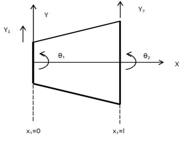MODELING OF GRADUAL DECREASE BEAM Linearly gradual decrease Beam element The beam element is assumed to be associated with two degrees of freedom, one rotation and one translation at each node. The location and positive directions of these displacements in a typical linearly gradual decrease Beam element are shown in Fig. 3.1 Some commonly used cross-sectional shapes of beams are shown in Table 3.1. The depth of the cross sections at http://www.iaeme.com/IJMET/index.asp 432 editor@iaeme.com Study & Vibration Analysis of gradual decrease Beam by FEM ends are represented by h1 (at free end) and h0 (at fixed end) similarly the width at the both ends are represented by b1 (at free end) and b0 (at fixed end) respectively. The length of the element is l. The axis about which bending is assumed to take place is indicated by a line in the middle coinciding with the neutral axis. Figure 1 The location and positive directions of these displacements in a typical linearly gradual decrease Beam element. For most of the beam shapes the variation in cross-sectional area along the length is represented by the following equation 1 The variation in the moment of inertia along the length about the axis of bending is given as 1 Where 1 Ax and Ix are the cross sectional area and moment of inertia at distance x from the small end; A1 and I1 and A0 and I0 are the cross sectional area and moment of inertia at free end and fixed end; and m and n refer to the corresponding shape factors that depends on the crosssectional shape and dimensions of the beam. The shape factors can be evaluated theoretically by observing the Eq. (3.1) and (3.2). Now by applying the condition for the beam as Ax=A0 and Ix=I0 at x=l, the condition gives the following equation In In , In In Thus, the shape factors can be found easily irrespective of the cross-section using the dimensions of at the two ends. Calculation of values of shape factors (m and n) from Eq. 3. 4 reveals that the expressions for Ax and Ix are exact at both ends of the beam. In some cases as for beams of I-section (Table 3.1), it has been found that, at points in between along the beam, Ax and Ix will deviate slightly from true values. The degree of this deviation is very small and for beams of all usual proportions, Eq. 3.1 and 3.2 gives values of area and moment of inertia at every section along the beam within one percent of deviation, which can be neglected, of the exact values. The shape factors m and n are dimensionless quantities; m and n varies between the limits 2.2-2.8. http://www.iaeme.com/IJMET/index.asp 433 editor@iaeme.com Mani Kant and Dr. Prabhat Kumar Sinha For theoretical analysis a rectangular cross-sectioned beam with linear variable width and depth is considered. Formulation of governing differential equation of gradual decrease Beam A general Euler’s Bernoulli beam is considered which is tapered linearly in both horizontal as well as in vertical planes. Fig. 3.2 shows the variation of width and depth in top and front view. The fundamental beam vibrating equation for Bernoulli-Euler is given by " ! ! 0 $ # The width and depth are varying linearly given by & &) '& ⁄ ', ) ) ) '& ⁄ ' Similarly area and moment of inertia will be varying accordingly &) & ' [ & '& ⁄ '][) ) '& ⁄ '], 1 & ' &) [) ) '& ⁄ '][ & '& ⁄ ']12 All the expressions for the beam area and moment of inertia at any cross-section are written after considering the variation along the length to be linear. Where ρ is the weight density, A is the area, and together ‘ρA/g’ is the mass per unit length, E is the modulus of elasticity and ‘I’ is the moment of inertia and l is the length of the beam. Here we considered only the free vibration, so considering the motion to be of form y(x, t) =z(x) sin (ωt), so applying the following relation to the fundamental beam equation we get . " ! &/ .' # Substituting Eq. (3.7) and (3.8) into (3.4), and by letting u = x/l (where u varies from 0 to 1) the following equation is obtained ' ) ' 3& &) 0 1 . 20 - . 3 5 1 & &) '2 ) ) '2 02 02 &) & 60 . ) '& ' ' 7 8 &) & & '2] [ '2] ) '2][ 02 [) 12 1 Ω 1 3 5 . # [ℎ + (ℎ − ℎ )2] By proper approximation i.e. α=h0/h1 and β=b0/b1 and k 12/ / # gets transformed into Eq. 11 (; − 1) 0 1 . 20 - . 3&: 1) 3 + 5 1 02 02 1 + (: − 1)2 1 + (; − 1)2 (; − 1)(: − 1) (: − 1) 60 . + 7 + 8 02 [1 + (: − 1)2][1 + (; − 1)2] [1 + (: − 1)2] ( <) . 8 =7 [1 + (: − 1)2] above equation The Eq. 3.10 is the final equation of motion for a double-tapered beam with rectangular cross-section. It was solved by numerical integration to give values of (lk) for various taper ratios for clamped-free beam with boundary conditions i.e. at x= 0 or u = 0, d2z/du2= 0 and z= http://www.iaeme.com/IJMET/index.asp 434 editor@iaeme.com Study & Vibration Analysis of gradual decrease Beam by FEM 0, at x= l or u= 1, dz/du= 0 and z= 0. This after solving leads to = < ℎ = >? @ . The relation can be used as a comparison while solving with FEA to show the effect of taper ratio on the fundamental frequencies and mode shapes. 3. FINITE ELEMENT ANALYSIS Most numerical techniques lead to solutions that yield approximate values of unknown quantities i.e. displacements and stiffness, only at selected points in a body. A body can be discretized into an equivalent system of smaller bodies. The assemblage of such bodies represents the whole body. Each subsystem is solved individually and the results so obtained are then contained are then combined to obtain solution for the whole body. It is applicable to wide range of problems involving non-homogeneous materials, nonlinear stress-strain relations, and complicated boundary conditions. Such problems are usually tackled by one of the three approaches, namely (i) displacement method or stiffness method (ii) the equilibrium or force method and (iii) mixed method. The displacement method, to which we shall confine our discussion, is widely used because of the simplicity with which it can be handled on the computer. In the displacement approach, a structure is divided into a number of finite elements and the elements are interconnected at joints called as nodes. The displacements in each element are then represented by simple functions. A displacement function is generally expressed in terms of polynomial. From the convergence point of view such a function is so chosen that it 1. Is continuous within the elements and compatible between the adjacent elements. 2. It includes the rigid body displacements and rotations of an element. 3. Has a consistent strain state. Further while choosing the polynomial for the displacement function, the order of the polynomial has to be chosen very carefully. Shape function The analysis of two dimensional beams using finite element formulation is identical to matrix analysis of structures. The Euler-Bernoulli beam equation is based on the assumption that the plane normal to the neutral axis before deformation remains normal to the neutral axis after deformation. Since there are four nodal variables for the beam element, a cubic polynomial function for y(x), is assumed as ( )=A +A +A + A- From the assumption for the Euler-Bernoulli beam, slope is computed from Eq. (3.1) is B( ) = A + 2A + 3CWhere α0, α1, α2, α3 are the constants The Eq. (3.1) can be written as : : - ] D E, Y(x) = [C][:] & ' [1 : :Where, : : - ]and[α]= D E [C] = [1 : :- http://www.iaeme.com/IJMET/index.asp 435 editor@iaeme.com Mani Kant and Dr. Prabhat Kumar Sinha For convenience local coordinate system is taken x1=0, x2=l that leads to A ;B A ; A A A A- - ; B A A A- This can be written as : 1 0 0 0 B : 0 1 0 0 I J I J D: E 1 :B 0 1 2 3 KAL = [ ]K:L, K:L = [ ]M KAL Eq. (4.3) can be written as N( ) = [O][ ]M KAL N( ) = [P]KAL Where [H] = [C] [A]-1 1 0 0 0 S 0 1 0 0 V R−3 −2 3 −1U U [ ]M = R R U 1 −2 −1U R2 Q T [H] = [H1(x), H2(x), H3(x), H4(x)] Where Hi(x) are called as Hermitian shape function whose values are given below P ( )= 1− - W XW + Y XY ,P ( ) = − X W + Y XW ,P ( )= Stiffness calculation of gradual decrease Beam - W XW − Y XY , P- ( ) = − W X + Y XW The Euler-Bernoulli equation for bending of beam is !+" ! = Z( , $) $ Where y(x, t) is the transverse displacement of the beam is the mass density, EI is the beam rigidity, q(x, t) is the external pressure loading, t and x represents the time and spatial axis along the beam axis. We apply one of the methods of the weighted residual, Galerkin’s method, to the above beam equation to develop the finite element formulation and the corresponding matrices equations. The average weighted residual of Eq. (4.10) is =[ " $ + ( ) ! − Z! \0 = 0 Where l is the length of the beam and p is the test function. The weak formulation of the Eq. (4.11) is obtained from integration by parts twice for the second term of the equation. Allowing discretization of the beam into number of finite elements gives = ]D [ " bc Where ^_ \0 + [ ^_ `=− a=− \ ( ) ( )d ( ) http://www.iaeme.com/IJMET/index.asp dY e dW e d W Y 0 − [ Z\0 E + 3−`\ − a ^_ 0\ 5 =0 0 is the shear force, is the bending moment, 436 editor@iaeme.com Study & Vibration Analysis of gradual decrease Beam by FEM fg is an element domain and n is the number of elements for the beam. 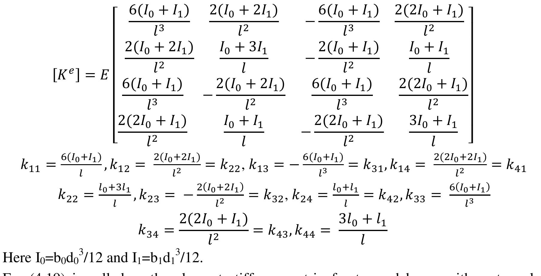Applying the Hermitian shape function and the Galerkin’s method to the second term of the Eq. (4.12) results in stiffness matrix of the gradual decrease Beam element with rectangular cross section i.e. X [i ] = [[j]k g ( )[j]0 [j] = KP " P " P " P-" L And the corresponding element nodal degree of freedom vector K0 g L = K B B Lk In Eq. (4.14) double prime denotes the second derivative of the function. Since the beam is assumed to be homogeneous and isotropic, so, E that is the elasticity modulus can be taken out of the integration and then the Eq. (4.13) becomes < <- <1 < < < < - < 1 ig = I J <- <- <-- <-1 <1 <1 <1- <11 Where kmn (m, n = 1, 4) are the coefficients of the element stiffness matrix. Where =< < X = [ ( ) P P 0 Solving the above equation, we get the respective values of coefficients of the element stiffness matrix for rectangular cross-sectioned beam. 6( + ) 2( + 2 ) 6( + ) 2(2 + ) S V − R U +3 + 2( + ) R 2( + 2 ) U − R U g [i ] = R 6( + ) 6( + ) 2(2 + )U 2( + 2 ) R U − R U + 3 + 2(2 + ) R2(2 + ) U − Q T < = m( n ) < X = ,< X n-X X = ,< ( n - XW = − <-1 = ) =< ,< ( n XW ) - =− = <- , < 2(2 + ) m( n ) 1 XY = = <1- , <11 = = <- , < X nX X 1 = ( = <1 , <-- = 3 + n ) XW m( n ) XY = <1 Here I0=b0d03/12 and I1=b1d13/12. Eq. (4.19) is called as the element stiffness matrix for tapered beam with rectangular cross-sectioned area. http://www.iaeme.com/IJMET/index.asp 437 editor@iaeme.com Mani Kant and Dr. Prabhat Kumar Sinha Mass matrix of gradual decrease Beam Since, for dynamic analysis of beams, inertia force needs to be included. In this case, transverse deflection is a function of x and t. the deflection is expressed with in a beam element is given below ( , $) = P ( ) ($) + P ( )B ($) + P ( ) ($) + P- ( )B- ($) ag = " D - - - 1 1 The coefficients of the element stiffness matrix are X 1 1 E -1 -1- 11 = [ ( )[P]k [P] 0 = (10 + 3 ) (15 + 7 ) 9( + ) (7 + 6 ) S V 35 420 140 420 R U (3 + 5 ) (6 + 7 ) ( + ) U R (15 + 7 ) R U 420 840 420 280 [ag ] = " R 9( + ) (6 + 7 ) (10 + 3 ) (15 + 7 )U R U 140 420 35 420 R U ( + ) (15 + 7 ) (5 + 3 ) U R (6 + 7 ) Q T 420 280 420 840 The above equation is called as consistent mass matrix, where the individual elements of the consistent mass matrices are = = XY (- nt w1 X( -t ) , - -1 = ) n- , = = XW (m 1 1 XW ( t = nu 1 = , 1 (7 + 6 ) = 1 420 And XW ( t nu ) = ) = ) nu - , 1- , 1 = 11 XY ( = The equation of motion for the beam can be written as [a]x0y z + [i]K0L = 0 = - n w XY (t ) = n- w1 vX( ) ) n 1 1 , = -- - = X( , n- -t ) , We seek to find the natural motion of system, i.e. response without any forcing function. The form of response or solution is assumed as K0($)L = K∅Le}~• Here {∅} is the mode shape (eigen vector) and ω is the natural frequency of motion. In other words, the motion is assumed to be purely sinusoidal due to zero damping in the system. The general solution turned out to be a linear combination of each mode as K0&$'L c K∅ Le}~ • c K∅ Le}~W • … … … . . cƒ K∅ƒ Le}~„ • Here each constant (ci) is evaluated from initial conditions. Substituting Eq. (4.27) into Eq. (4.25) gives & / [a] [i]'K∅Le}~• 0 Using the above equation of motion for the free vibration the mode shapes and frequency can be easily calculated. http://www.iaeme.com/IJMET/index.asp 438 editor@iaeme.com Study & Vibration Analysis of gradual decrease Beam by FEM Numerical analysis For numerical analysis a taper beam is considered with the following properties: Material properties Elastic modulus of the beam = 2.109e11 N/m2 Density = 7995.74 Kg/m3 Fundamental frequencies for free vibration analysis is calculated by using the equation of motion described in the previous section for two end conditions of beam given below 1. One end fixed and one end free (cantilever beam) 2. 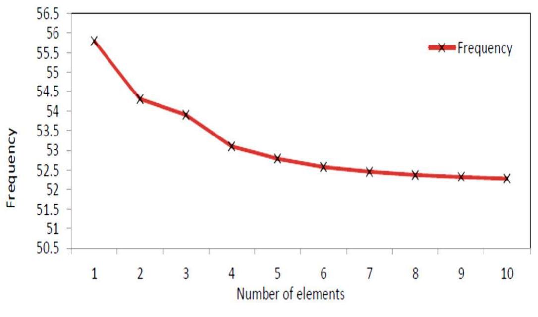Simply supported beam Calculation of frequency of cantilever beam After discretizing to 10 numbers of elements, natural frequencies of the gradual decrease Beam are calculated using MATLAB program and shown in Table 5.1. As we can see in Fig. 5.3 the frequency converges after discretizing to only four elements. The results are compared with Mabie [1] and Gupta [9] who solved the final differential equation for the beam using numerical method. The method described in here is less cumbersome than the conventional methods. Table 1 Frequencies of linearly tapered cantilever beam. Frequency (cycles/sec) 1 2 3 4 5 6 7 8 9 10 11 12 13 14 15 16 17 18 19 20 Number of Elements 1 2 3 55.8 54.3 53.9 460.48 411.22 403.3 1288.5 1186.8 4652.9 2755.6 5198.1 11479.2 4 53.1 398.29 1178.6 2642.6 4440.8 7147.4 11345.8 20968.4 http://www.iaeme.com/IJMET/index.asp 5 6 7 8 9 52.79 52.58 52.46 52.38 52.33 395.82 394.4 393.61 393.16 392.68 1169.08 1163.8 1160.89 1159 1157.77 2334.3 2318 2308.2 2302 2298.6 3888.7 3879.1 3854.6 3837 3827.1 6536.36 5828.4 5813.5 5780 5754.6 9587.54 9037.5 8165.1 8137 8097.4 13910.9 12466.5 11940.2 10902 10851.5 19789.1 17045.5 15769.6 15240 14045.3 33176 23033 20661 19491 18933 30414 26849 24725 23628 48142 34445 31172 29222 43176 38075 35969 65882 56400 44015 54112 53412 64192 63813 69022 79985 439 10 52.29 392.4 1156.8 2296.1 3820.2 5737.1 8060.8 10805 13955 17595 23017 28178 34142 41217 49527 59179 70065 81661 94367 135776 editor@iaeme.com Mani Kant and Dr. 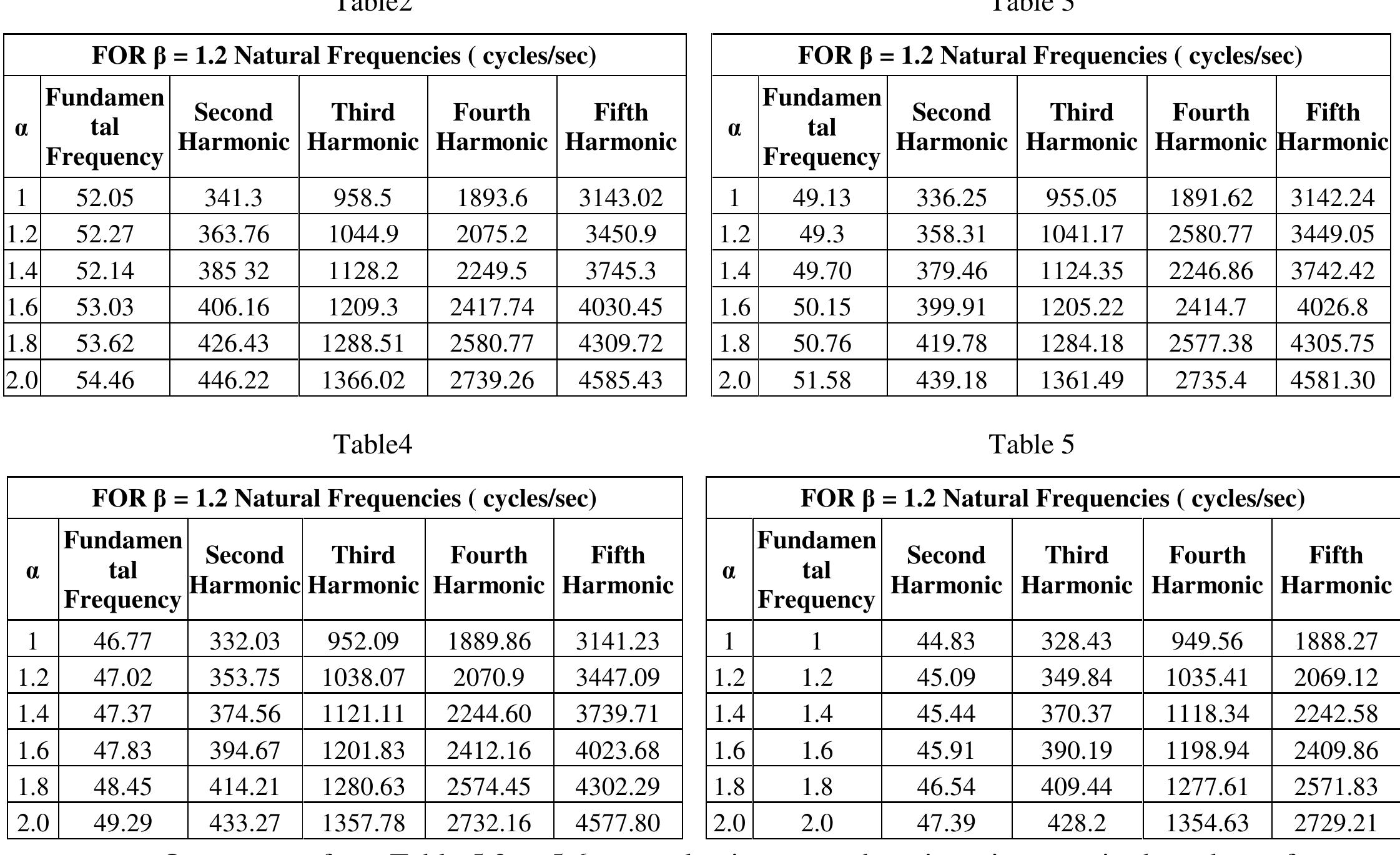Prabhat Kumar Sinha Figure 2 Convergence of fundamental natural frequency for cantilever beam Effect of taper ratio on the frequency For determining the effect of taper ratio on the frequency, different values of α (depth variation) and β (width variation) varying from 1 to 2 are taken in consideration and shown in Tables Frequencies of Linearly Tapered Cantilever Beam for different values of α and β. Table2 Table 3 FOR β = 1.2 Natural Frequencies ( cycles/sec) α Fundamen Second Third Fourth Fifth tal Harmonic Harmonic Harmonic Harmonic Frequency 1 1.2 1.4 1.6 1.8 2.0 52.05 52.27 52.14 53.03 53.62 54.46 341.3 363.76 385 32 406.16 426.43 446.22 958.5 1044.9 1128.2 1209.3 1288.51 1366.02 1893.6 2075.2 2249.5 2417.74 2580.77 2739.26 3143.02 3450.9 3745.3 4030.45 4309.72 4585.43 FOR β = 1.2 Natural Frequencies ( cycles/sec) α 1 1.2 1.4 1.6 1.8 2.0 Fundamen Second Third Fourth Fifth tal Harmonic Harmonic Harmonic Harmonic Frequency 49.13 49.3 49.70 50.15 50.76 51.58 336.25 358.31 379.46 399.91 419.78 439.18 Table4 1 1.2 1.4 1.6 1.8 2.0 Fundamen Second Third Fourth Fifth tal Harmonic Harmonic Harmonic Harmonic Frequency 46.77 47.02 47.37 47.83 48.45 49.29 332.03 353.75 374.56 394.67 414.21 433.27 952.09 1038.07 1121.11 1201.83 1280.63 1357.78 1891.62 2580.77 2246.86 2414.7 2577.38 2735.4 3142.24 3449.05 3742.42 4026.8 4305.75 4581.30 Table 5 FOR β = 1.2 Natural Frequencies ( cycles/sec) α 955.05 1041.17 1124.35 1205.22 1284.18 1361.49 1889.86 2070.9 2244.60 2412.16 2574.45 2732.16 3141.23 3447.09 3739.71 4023.68 4302.29 4577.80 FOR β = 1.2 Natural Frequencies ( cycles/sec) α 1 1.2 1.4 1.6 1.8 2.0 Fundamen Second Third Fourth Fifth tal Harmonic Harmonic Harmonic Harmonic Frequency 1 1.2 1.4 1.6 1.8 2.0 44.83 45.09 45.44 45.91 46.54 47.39 328.43 349.84 370.37 390.19 409.44 428.2 949.56 1035.41 1118.34 1198.94 1277.61 1354.63 1888.27 2069.12 2242.58 2409.86 2571.83 2729.21 One can see from Table 5.3 to 5.6 as α value increases there is an increase in the values of fundamental frequency, but the taper ratio β in the horizontal plane has a detrimental effect on frequency. http://www.iaeme.com/IJMET/index.asp 440 editor@iaeme.com Study & Vibration Analysis of gradual decrease Beam by FEM Mode shapes To determine the effect of β and α on the amplitude of vibration, their values are varied (1 to 2) and mode shapes are calculated and shown in Fig. Figure 3 Figure 4 Figure 5 Figure 6 Figure 7 Figure 8 http://www.iaeme.com/IJMET/index.asp 441 editor@iaeme.com Mani Kant and Dr. Prabhat Kumar Sinha Figure 9 Figure 10 There are four different modes shape for cantilever beam with constant width (β) and variable depth ratio (α) Maximum values of amplitude is taken for each mode and for different values of taper ratios the % age reduction in amplitude with respect to no taper is calculated, As one can see from Table 2 to 5, the effect of α on decreasing the amplitude is quite more than β. 4. CONCLUSIONS This research work presents a simple procedure to obtain the stiffness and mass matrices of tapered Euler’s Bernoulli beam of rectangular cross section. The proposed procedure is verified by the previously produced results and method. The shape functions, mass and stiffness matrices are calculated for the beam using the Finite Element Method, which requires less computational effort due to availability of computer program. The value of the natural frequency converges after dividing into smaller number of elements. It has been observed that by increasing the taper ratio ‘α’ the fundamental frequency increases but an increment in taper ratio‘β’ leads to decrement in value of fundamental frequency. Mode shapes for different taper ratio has been plotted. Taper ratio‘α’ is more effective in decreasing the amplitude in vertical plane, than β in the horizontal plane at higher mode. The above result is of great use for structural members where high strength to weight ratio is required. REFERENCES [1] [2] [3] [4] [5] [6] H. H. Mabie & C. B. Rogers, Transverse vibrations of double-tapered cantilever beams, Journal of the Acoustical Society of America 36, 463-469, 1964. H. H. Mabie and C. B. Rogers, Transverse vibrations of tapered cantilever beams with end support, Journal of the Acoustical Society of America, 44, 1739-1741, 1968. G.R. Sharp, M.H. Cobble, Finite transform solution of the vibrating beam with ends elastically restrained, Journal of the Acoustical Society of America, 45, 654–660, 1969. W. Carnegie & J. Thomas, The coupled bending-bending vibration of pre-twisted tapered blading, Journal of Engineering for Industry 94(1), 255 -267, 1972. K.R. Chun, Free vibration of a beam with one end spring-hinged and the other free, Journal of Applied Mechanics, 39, 1154–1155, 1972. R.P. Goel, Vibrations of a beam carrying a concentrated mass, Journal of Applied Mechanics, 40, 821–822, 1973. http://www.iaeme.com/IJMET/index.asp 442 editor@iaeme.com Study & Vibration Analysis of gradual decrease Beam by FEM [7] [8] [9] [10] [11] [12] [13] [14] [15] [16] [17] [18] [19] [20] [21] [22] [23] [24] [25] [26] K.J. Bathe, E.L. Wilson, F.E. Peterson, A structural analysis system for static and dynamic response of linear systems,” College of Engineering, University of California, Report EERC 73-11, 1973. R.C. Hibbeler, Free vibration of a beam support by unsymmetrical spring-hinges, Journal of Applied Mechanics, 42, 501–502, 1975. A. K. Gupta, Vibration Analysis of Linearly Gradual decrease Beam s Using FrequencyDependent Stiffness and Mass Matrices, thesis presented to Utah State University, Logan, Utah, in partial fulfillment of the requirements for the degree of Doctor of Philosophy, 1975. K. Kanaka Raju, B. P. Shastry, G. Venkateswarraa, A finite element formulation for the large amplitude Vibrations of gradual decrease Beam s, Journal of Sound and Vibration, 47(4), 595-598 1976. R. S. Gupta & S. S. Rao, Finite element Eigen value analysis of tapered and twisted Timoshenko beams J. Sound Vibration, 56, 187-200, 1978. C. D. Bailey Direct analytical solutions to non-uniform beam problems, Journal of Sound and Vibration, 56(4), 501-507, 1978. C. W. S. To, Higher order gradual decrease Beam finite elements for vibration analysis Journal of Sound and Vibration, 63(I), 33-50, 1979. J.H. Lau, Vibration frequencies of tapered bars with end mass, Journal of Applied Mechanics, 51, 179–181, 1984 J.R. Banerjee, F.W. Williams, Exact Bernoulli-Euler static stiffness matrix for a range of gradual decrease Beam -columns, International Journal for Numerical Methods in Engineering 23, 1615-1628, 1986. M.A. Bradford, P.E. Cuk, Elastic buckling of tapered mono-symmetric I-beams, Journal of Structural Engineering ASCE 114 (5), 977-996, 1988. E. Howard Hinnant, Derivation of a Tapered p-Version Beam Finite Element, NASA Technical Paper 2931 AVSCOM Technical Report, 89-B-002, 1989. K. M. Liew, M. K. Lim and C. W. Lim, Effects of initial twist and thickness variation on the vibration behavior of shallow conical shells, Journal of Sound and Vibration, Volume 180, Issue 2, 16 February, 271–296, 1995. T.D. Chaudhari, S.K. Maiti, Modelling of transverse vibration of beam of linearly variable depth with edge crack, Engineering Fracture Mechanics, 63, 425-445, 1999. N. Bazeos, D.L. Karabalis, Efficient computation of buckling loads for plane steel frames with tapered members, Engineering Structures, 28, 771-775, 2006. Mehmet Cem Ece, Metin Aydogdu, Vedat Taskin, Vibration of a variable cross- section beam, Mechanics Research Communications, 34, 78–84, 2007. B. Biondi, S. Caddemi, Euler-Bernoulli beams with multiple singularities in the flexural stiffness, European Journal of Mechanics A-Solids, 26, 789-809, 2007. J.B. Gunda, A.P. Singh, P.S. Chhabra and R. Ganguli, Free vibration analysis of rotating tapered blades using Fourier-p super element, Structural Engineering and Mechanics, Vol. 27, No. 2 000-000, 2007. A. Shooshtari & R. Khajavi, An efficient procedure to find shape functions and stiffness matrices of non-prismatic Euler Bernoulli and Timoshenko beam elements, European Journal of Mechanics, 29, 826-836c. 2010. Tayeb Chelirem and Bahi Lakhdar, Dynamic study of a turbine tapered blade, Science Academy Transactions on Renewable Energy Systems Engineering and Technology (SATRESET), Vol. 1, No. 4, , ISSN: 2046-6404, (2011) Reza Attarnejad and Ahmad Shahba, Basic displacement functions for centrifugally stiffened gradual decrease Beam s, International Journal numerical Methods Biomedical engineering, 27:1385–1397, 2011. http://www.iaeme.com/IJMET/index.asp 443 editor@iaeme.com Mani Kant and Dr. Prabhat Kumar Sinha [27] [28] [29] [30] [31] Reza Attarnejad, Ahmad Shahba, Dynamic basic displacement functions in free vibration analysis of centrifugally stiffened gradual decrease Beam s, Meccanica, 46:1267– 1281, 2011. P. Henri Gavin, Structural element stiffness matrices and mass matrices, Department of Civil and Environmental Engineering CEE 541 Structural Dynamics, 2012. Fig. 2 Cantilever Beam of rectangular cross-section area with width and depth varying linearly. Prince Kumar and Sandeep Nasier, An Analytic and Constructive Approach to Control Seismic Vibrations in Buildings. International Journal of Civil Engineering and Technology, 7(5), 2016, pp.103–110. G. Thulasendra and U.K. Dewangan, Comparative Study of Vibration Based Damage Detection Methodologies For Structural Health Monitoring, International Journal of Civil Engineering and Technology, 8(7), 2017, pp. 846–857. S. Jayavelu, C. Rajkumar, R. Rameshkumar and D. Surryaprakash, Design and Analysis of Vibration and Harshness Control For Automotive Structures Using Finite Element Analysis, International Journal of Civil Engineering and Technology, 8(10), 2017, pp. 1364–1370. http://www.iaeme.com/IJMET/index.asp 444 editor@iaeme.com