Geophysical fluid dynamics

Introduction

Low-order models (LOMs) reveal basic mechanisms and their interplay through the focus on key elements and retaining only minimal number of degrees of freedom. Following the pioneering work by Lorenz (1960Lorenz ( , 1963 and Obukhov (1969), they have been widely employed in studies of atmospheric dynamics and turbulence (e.g., Lorenz, 1972Lorenz, , 1982Lorenz, , 2005Obukhov, 1973;Obukhov and Dolzhansky, 1975;Charney and DeVore, 1979;Källén and Wiin-Nielsen, 1980;Legra and Ghil, 1985;Yoden, 1985;Howard and Krishnamurti, 1986;Shirer, 1987;De Swart, 1988;Gledzer et al., 1988;Tsonis, 1992;Wiin-Nielsen, 1992;Frisch, 1995;Roebber, 1995;Bokhove and Shepherd, 1996;Holmes et al., 1996;Kwasniok, 1997Kwasniok, , 2004Bohr et al., 1998, Majda andTimofeyev, 2000;Van Veen et al., 2001;Koo and Ghil, 2002;Majda et al., 2003;Biferale, 2003;Lakshmivarahan et al., 2003;Maas, 2004;Roebber and Tsonis, 2005). LOMs are commonly derived from the original PDEs by employing the Galerkin method: fluid dynamical fields are expanded into Correspondence to: A. Gluhovsky ([email protected]) infinite sets of time-independent basis functions; then projection of the PDEs onto these functions yields a finite system of ODEs (the LOM) for the time evolution of the coefficients in truncated expansions.

The method, however, does not provide criteria for selecting modes, while in arbitrary truncations fundamental conservation properties of the fluid dynamical equations may be violated, resulting in LOMs with unphysical behaviors (throughout the paper "conservation" means "conservation in the absence of forcing and dissipation"). This has been demonstrated, in particular, by attempts to extend the celebrated Lorenz (1963) (1) A common misconception is that modal truncations will always conserve quadratic invariants of the original equations. This is not the case when the forcing is thermal (such as fixed temperatures at the boundaries in Rayleigh-Bénard convection) thus coupling the momentum and heat equations. For example, the important and widely discussed Howard-Krishnamurti (1986) model of convection with shear lacks energy conservation and, as a result, has trajectories going to infinity. Thiffeault and Horton (1996) restored energy conservation in the model by adding a term to the Galerkin temperature expansion. Hermiz et al. (1995) noted that the Howard-Krishnamurti (1986) model lacked total vorticity conservation, which they remedied by adding a term to the streamfunction expansion. Their model, however, still lacked energy conservation. Another example of a LOM lacking energy conservation is the model of 3-D Rayleigh-Bénard convection by Das et al. (2000) (see Sect. 2.2.2 below).

To avoid unphysical behaviors, it was proposed (Gluhovsky, 1982(Gluhovsky, , 1986a to construct LOMs in the form of coupled 3-mode nonlinear systems known in Published by Copernicus GmbH on behalf of the European Geosciences Union and the American Geophysical Union.

126

A. Gluhovsky: Energy-conserving and Hamiltonian low-order models mechanics as Volterra gyrostats (Volterra, 1899; see also Wittenburg, 1977),

(2) Gyrostat (Eq. 2) can be thought of as a rigid body containing an axisymmetric rotor that rotates with a constant angular velocity about an axis fixed in the carrier. In this interpretation, I i , i=1, 2, 3, are the principal moments of inertia of the gyrostat, ω is the angular velocity of the carrier body, and h is the fixed angular momentum caused by the relative motion of the rotor (the gyrostatic motion). The development of LOMs in the form of coupled gyrostats is based on Obukhov's modular approach to constructing LOMs (Obukhov, 1973;Obukhov and Dolzhansky, 1975) and on the following findings: (i) Lorenz model (Eq. 1) is actually the simplest Volterra gyrostat (within the vertical bars in Eqs. (3) below, we call it the "Lorenz gyrostat") with added constant forcing and linear friction (Gluhovsky, 1982),

i.e., Eqs. (3) may be converted into Eqs. (1) by a linear change of variables. (ii) Effective existing LOMs for atmospheric circulations and turbulence can be transformed into coupled gyrostats (Gluhovsky 1986a, b). (iii) LOMs that do not have a gyrostatic form typically do not retain the energy conservation property of the original equations, which results in unphysical behavior (Gluhovsky and Tong, 1999). The discussed above Howard-Krishnamurti (1986) model cannot be converted to coupled gyrostats, but its modification that conserves both energy and total vorticity is a system of coupled gyrostats (Gluhovsky et al., 2002). Lorenz (1960) and Obukhov (1969) insisted that a LOM should retain conservation properties of the original equations. Obukhov (1969) showed that the simplest such LOM is equivalent to the Euler rigid body (system (2) without its linear terms), which was also derived by Lorenz (1960) as the simplest model of atmospheric dynamics. As noted by Arnold (1991), similar 3-mode LOMs were introduced by Kolmogorov in 1958 at his seminar on dynamical systems. Pasini and Pelino (2000) discuss Kolmogorov and Lorenz systems in a geometric framework. Obukhov also suggested systems of coupled Euler gyroscopes for modeling homogeneous flows (Obukhov, 1973). The linear terms in Eqs. (2) are caused by the relative motion of the rotor. Unlike linear viscous terms, they do not affect the conservation of energy or phase space volume. In LOMs, they occur due to various "inhomogeneous" factors peculiar to geophysical fluid dynamics (stratification, rotation, and topography) (Gluhovsky 1986a, Gluhovsky andTong, 1999).

Restricting LOMs to have a gyrostatic form 1) ensures energy conservation, thus preventing certain unphysical behav-iors; 2) provides for optimal mode selection (resulting in the smallest LOM that still describes the effect of interest); 3) allows a modular implementation of the Galerkin technique with gyrostats as elementary building blocks (see, Gluhovsky et al., 2002). At the same time, gyrostatic truncations do not in general capture the Hamiltonian structure of the original equations, which may allow for other unphysical behaviors. For example, the mentioned above energy-conserving modification by Thiffeault and Horton (1996) of Howard-Krishnamurti (1986) model can be converted to couple gyrostats (Gluhovsky and Tong (1999), but it still lacks the vorticity conservation. This may also have unpleasant consequencies, such as "that the rigid boundaries act as a constant virticity sink" (Hermitz et al., 1995).

Since the conservative part of various models in geophysical fluid dynamics (the primitive equations, shallow water equations, quasi-geostrophic equations) is Hamiltonian, the most consistent way to retain in a LOM the fundamental conservation properties of the original system is through maintaining the Hamiltonian structure (Salmon, 1983(Salmon, , 1988Shepherd, 1990). Note that gyrostat (Eq. 2) has two quadratic invariants (the kinetic energy, E= I i ω 2 i /2, and the square of the angular momentum, C= (I i ω i +h i ) 2 ), and may be presented in the Hamiltonian form,

where

∂M j , and Casimir invariant C. Although modal truncations generally destroy the Hamiltonian structure (the Jacoby property Eq. 23) so that it is difficult (and often believed impossible) to develop a Hamiltonian LOM with more than 3-modes for a problem at hand (see, however, Zeitlin, 1991), it will be demonstrated in this paper how gyrostatic LOMs become instrumental in constructing Hamiltonian multi-mode LOMs.

In Sect. 2, gyrostatic LOMs originating from the Rayleigh-Bénard convection (RBC) are reviewed. In Sect. 3, some of these LOMs are shown to be Hamiltonian. Being of fundamental importance in nonlinear dynamics where it is the most carefully studied example of nonlinear systems exhibiting self-organization and transition to chaos, RBC promotes understanding of many real-world fluid flows as well, sharing a number of important properties with other pattern-forming processes (Getling, 1998). RBC is the principal mechanism of mesoscale shallow convection (Agee, 1987;Atkinson and Zhang, 1996), it is also important for studies of flows in other geophysical fluids (in the oceans, in the liquid core of the Earth) and in astrophysics (e.g., Meyer-Spasche, 1999). At the same time, from both experimental and theoretical point of view RBC is a particularly simple and accessible case of convection, which is the prevalent type of fluid motion in the Universe (Emanuel, 1994). Thus, the gyrostatic approach illustrated below with LOMs of the RBC has a considerably wider applicability. In Sect. 4, new areas are outlined where LOMs in the form of coupled gyrostats may be useful.

A. Gluhovsky: Energy-conserving and Hamiltonian low-order models 127 2 Gyrostatic LOMs for Rayleigh-Bénard convection The Rayleigh-Bénard problem deals with the convective overturning that occurs in a fluid heated from below. The fluid is confined between two horizontal planes z=0 and z=H maintained at constant temperatures: T 0 at the lower surface and T 0 − T at the upper one. It is commonly described by the Boussinesq equations (e.g., Chandrasekhar, 1961),

where u is the velocity, g is the gravitational acceleration, p is the pressure, ρ 0 is the density at temperature T 0 , ε is the coefficient of thermal expansion, and ν and κ are the coefficients of kinematic viscosity and thermal diffusivity, respectively. Horizontal periodic boundary conditions with period 2L are assumed. The nondimensional parameters for the problem are the Rayleigh number Ra=g ε T H 3 /κ ν characterizing the relative importance of the thermal buoyancy and the stabilizing effect of diffusion, and the Prandtl number P r=ν/κ describing the relative importance of viscous and thermal diffusion.

For developing LOMs in the form of coupled gyrostats, it is convenient to write Eqs. (2) in terms of variables

LOMs in the form of coupled gyrostats possess a number of features shared with the Navier-Stokes equations (Gluhovsky, 1982;Gluhovsky and Tong, 1999) that Lorenz (1960Lorenz ( , 1972 and Obukhov (1969) consider desirable for LOMs: (1) They are quadratically nonlinear. (2) In the inviscid, unforced limit, they have at least one quadratic integral of motion (E= x 2 i /2, interpreted as some form of energy); they also conserve phase-space volume (since ∂ẋ i /x i =0, which implies the Liouville theorem). (3) Their solutions are bounded (even when there is linear viscous friction and constant forcing) (Gluhovsky and Tong, 1999).

LOMs for 2-D Rayleigh-Bénard convection

Extensions of Lorenz model (Eq. 1) have often yielded ambiguous results: for some combinations of modes a strange attractor appeared, while for other combinations it seemed to vanish. Treve and Manley (1982) introduced a consistent procedure for mode selection in the 2-D Rayleigh-Bénard problem producing energy conserving LOMs. Their l-order approximations for nondimensional stream function ψ(t, x, z) and the deviation from equilibrium vertical temperature profile θ(t, x, z) (the fluid is assumed to circulate in (x, z) plane with no motion in y-direction),

is defined by the first l terms of the ascending sequence,

of the eigenvalues ρ m,n =a 2 m 2 + n 2 of the linear problem that determines the basis functions for ψ(t, x, z). In Eqs. 7, the sums are over the set E of pairs {m i , n i } from Eq. (8), m i , n i >0, 1≤i≤l;n= max 1≤i≤l n i , and a=H /L (see Eqs. 5).

When sequence (8) is limited to ρ 1,1 , series (7) become most severely truncated to

(the mode corresponding to θ 0, 1 (t) decays exponentially). This results in the simplest LOM for 2-D Rayleigh-Bénard convection,

Then applying one linear change of variables transforms system (10) into Lorenz model (Eq. 1), while another such transformation leads to the LOM equivalent to Eqs. (3),

where the Lorenz gyrostat (3) has a particularly simple form (Gluhovsky, 1986b;Gluhovsky et al., 2002). Note that because our interest here is focused on the conservative part of equations, same symbols (F for the external force and α i for dissipative coefficients) are used in all LOMs throughout the paper, although the actual values of such constants are not the same in different models (e.g., LOM (3) and LOM (11)). In general, the LOM resulting from the Galerkin procedure based on expansions (7) can be presented as a multilayer system of coupled gyrostats (Gluhovsky, 1986b). Every layer of the system is composed of Lorenz gyrostats (of different time scales) having one common mode and corresponding to the eigenvalues with the same second index; for example, Lorenz gyrostats in the first layer correspond to ρ 1,1 , ρ 2,1 , ρ 3,1 , ..., those in the second layer correspond to ρ 2,1 , ρ 2,2 , ρ 3,2 , ..., etc. The layers are connected by subsystems of Euler gyroscopes (gyrostats 3 or 6 without linear terms). The number of Lorenz gyrostats in each layer and the number of layers are determined by the aspect ratio and the order of approximation. The approximation of order l will have only one layer if ρ l,1 ≤ρ 1,2 , i.e., a 2 l 2 +1<a 2 +4, or a< 3/(l 2 −1). For instance, the following LOM composed of three Lorenz gyrostats is a valid third-order approximation for 2-D Rayleigh-Bénard convection when a< √ 3/8:

where d k =k √ ρ 11 /ρ k1 . Note that gyrostats in LOM (12) are of different time scales d −1 k . Variables x 1 −x 7 are linearly related to θ 02 , θ 11 , ψ 11 , θ 21 , ψ 21 , θ 31 , ψ 31 , respectively, in expansions (7). As the order of approximation is increased by one, one more Lorenz gyrostat is added to the system.

LOMs for 3-D Rayleigh-Bénard convection

To obtain LOMs for 3-D Rayleigh-Bénard convection, Tong and Gluhovsky (2002) used the following Galerkin expansions for the dimensionless three components of the velocity and the temperature deviation from the conductive steady state profile,

cos ax sin z − av(t) cos ay sin z θ 002 (t) sin 2z + θ 101 (t) cos ax sin z + θ 011 (t) cos ay sin z +w(t) sin ax cos ay cos 2z, +w(t) cos ax sin ay cos 2z, −aw(t) cos ax cos ay sin 2z, +θ 112 (t) cos ax cos ay sin 2z + θ 004 (t) sin 4z. 13Lorenz (1963) modes are retained in expansions (13) for each horizontal direction, and interaction modes for velocity (w) and temperature (θ 112 ) are added as well as mode θ 004 whose role is explained in the end of Sect. 2.2.2.

An analog of Lorenz model (Eq. 1)

Considering only the expansions within the box in Eqs. (13) results in the simplest LOM of 3-D Rayleigh-Bénard convection,

the 3-D analog of the Lorenz model (Eq. 1), where two Lorenz gyrostats describe the dynamics in the (x, z) and (y, z) planes, respectively. In Eqs. 14, variables x 1 −x 5 are linearly related to θ 002 , θ 101 , u, θ 011 , v in expansions (13). When LOM (Eq. 12) is composed of two Lorenz gyrostats, it is similar to LOM (Eq. 14); the difference is that gyrostats in LOM (Eq. 12) are of different scales. Equations (14) may be considered from another angle. As revealed by Arnold (1966), when equations of Euler rigid body (Eqs. 2) without linear terms),

are viewed as a quadratically nonlinear system on the Lie algebra of the group SO(3) (the group of rotations of 3-D Euclidean space), they have natural analogs on arbitrary Lie algebras. The following quadratically nonlinear system on the Lie algebra of the group SO(n),

is called the n-dimensional rigid body. Equations (15) are obtained from Eqs. (16) by setting n=3 and denoting

Following this design, the n-dimensional gyrostat may be defined as the n-dimensional analog of Volterra equations (Eqs. 2):

Equations (2) result from Eqs. (18) by setting n=3 and adding to Eq. (17) h 1 =h 21 , h 2 =h 31 , h 3 =h 32 .

Equations for the forced regime are obtained by adding in each of Eqs. (18) the terms of the form −α ij ij +N ij , α ij =α j i >0, N ij =−N j i . For example, at n = 3, setting λ 2 =λ 3 , h 2 =h 3 =0 and N ij ≡0, except for N 21 =−N 12 =F , we get LOM (Eq. 3). At n=4, denote in addition to Eq. (17), ω 4 = 41 , ω 5 = 42 , ω 6 = 43 I 4 = λ 4 + λ 1 , I 5 = λ 4 + λ 2 , I 6 = λ 4 + λ 3 , α 1 = α 21 , α 2 = α 31 , α 3 = α 32 , α 4 = α 43 , α 5 = α 42 , α 6 = α 43 , (19) and set λ 2 =λ 3 =λ 4 , h ij =N ij ≡0, save for h 21 =−h 12 =h 1 , and

Then because of the symmetry condition λ 2 =λ 3 =λ 4 , the equation for ω 6 becomes I 3ω 6 =−α 6 ω 6 , i.e., ω 6 →0, while the equations for the remaining modes take the form of two coupled Lorenz gyrostats in the forced regime:

Finally, the linear change of variables,

converts Eqs. (20) into Eqs. (14). The dissipative coefficients α i in Eqs. 14are obtained from those in Eqs. 20as (C −1 I −1 1 ) α i for i=1, 2, 4, and (C −1 I −1 3 ) α i for i=3, 5, and constant F in Eqs. 14is calculated from that in Eqs. (20) as (AC −1 I −1 1 ) F . Thus, while the Lorenz model (Eq. 1) of 2-D Rayleigh-Bénard convection is a 3-dimensional (Volterra) gyrostat in the forced regime, its analog for the 3-D Rayleigh-Bénard convection may be considered as a 4-dimensional gyrostat in the forced regime.

An 8-mode LOM of 3-D Rayleigh-Bénard convection

When full expansions (13) are used, the Galerkin procedure results in the following LOM in variables x 1 −x 8 linearly related to θ 002 , θ 101 , u, θ 011 , v, θ 004 , θ 112 , w, respectively (Tong and Gluhovsky, 2002), 14and (21) exhibit behaviors peculiar to 3-D dynamics: steady state solutions (that include 2-D rolls in either x or y directions, symmetric square convection cells, and intermediate planforms), as well as periodic and chaotic regimes that may coexist in the same parameter region. However, due to severe truncation, steady state solutions in LOM (Eq. 14) have stability regions contradicting the experimental results. The larger LOM (Eq. 21) is free of these drawbacks and has a larger variety of regimes.

Excluding the θ 004 (t) sin 4z term in the temperature expansion (13), results in the seven-mode system by Das et al. (2000) that has pathological solutions exponentially diverging to infinity. This system cannot be converted to coupled gyrostats form: it turns out that nonlinear terms of gyrostat III in Eqs. (21) are absent while its linear terms have the same sign, causing violation of the energy conservation.

Hamiltonian LOMs

A finite-dimensional Hamiltonian dynamical system may be written (Shepherd, 1990;Morrison, 1998) aṡ

where H is the Hamiltonian function andJ is an antisymmetric matrix (J ij =−J j i ) that needs to satisfy the Jacobi conditions

(repeated indices imply summation). Thus, the search for Hamiltonian structure "should consist of identifying the fundamental objects x, H , and J , and demonstrating that J possesses the requisite abstract-algebraic properties" (Shepherd 1990). Gyrostatic LOMs are particularly helpful for developing Hamiltonian LOMs. First, they all conserve the phase-space volume and possess a constant of motion,

(representing some form of energy), which is a good candidate for the Hamiltonian function. Second, any system of coupled gyrostats is readily presented in form (22) with easily determined antisymmetric matrix J , for which it is pretty straightforward to check Jacobi conditions (Eqs. 23). If they are not met, one may try to reduce the LOM to a Hamiltonian one by deleting certain gyrostats (as demonstrated below with LOM (Eq. 21) reduced to a Hamiltonian LOM (Eq. 28)). The new reduced LOM is still a system of coupled gyrostats with an integral of motion of form (24) thus providing for an easy check of the Jacobi conditions.

The Volterra gyrostat

The first example is provided by Eqs. (6) that have Hamiltonian form (22) with H =(x 2 1 +x 2 2 +x 2 3 )/2 and antisymmetric matrix

obeying Jacobi conditions (Eq. 23). The system has one Casimir invariant corresponding to the conservation of the square of the angular momentum.

3.2 LOM (Eq. 12) for 2-D Rayleigh-Bénard convection with small aspect ratio

The conservative part of this LOM has Hamiltonian form

and Casimir invariant C= 1 2 x 2 3 +x 2 5 +x 2 7 +x 1 .

LOMS for 3-D Rayleigh-Bénard convection

Similarly, in the 3-D Rayleigh-Bénard problem, the conservative part of LOM (Eq. 14) (the 3-D analog of the Lorenz model) is Hamiltonian with H =

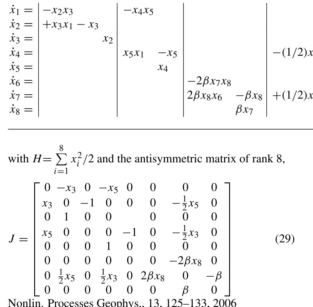
and Casimir invariant C= 1 2 x 2 3 +x 2 5 +x 1 . The larger LOM (Eq. 21) (without friction and forcing) is not Hamiltonian. However, by deleting gyrostat VI in Eqs. (21) we obtain a Hamiltonian LOM,

with H = 8 i=1

x 2 i /2 and the antisymmetric matrix of rank 8,

The Euler gyroscope in Eqs. (21) (gyrostat VI) may destroy the Hamiltonian property even when coupled with only one Lorenz gyrostat. To defend its removal, note that Galerkin method per se does not provide any guidance on the selection of modes to retain in the truncation, so that the presence of particular gyrostats in the resulting LOM, dependent on the choice of the retained modes, is therefore somewhat arbitrary. The idea behind the methodologies described in the manuscript is to select (via gyrostats) those modes that result in an energy-conserving LOM, then keep gyrostats that help retaining the Hamiltonian structure.

Concluding discussion

In this paper, an approach was described to the development of low-order models in geophysical fluid dynamics in the form of coupled gyrostats. Such systems always possess a quadratic integral of motion (interpreted as some form of energy), which eliminates certain unphysical behaviors that often plague LOMs obtained through ad hoc Galerkin truncations. At the same time, coupled gyrostats do not necessarily retain the Hamiltonian property of the original equations, which may allow for other unphysical behaviors. Yet, the gyrostatic structure was shown to provide for an easy development of multi-mode Hamiltonian LOMs, contrary to a widespread belief that only 3-mode truncations can be Hamiltonian. This is not a systematic procedure for derivation of Hamiltonian LOMs, but there is no general method for determining whether or not a system is Hamiltonian. The Hamiltonian property may be found too limiting for LOMs, and non-Hamiltonian LOMs are often quite successful. Still, stripped from many attributes of the original equations, it is desirable that, in general, LOMs should retain their fundamental properties.

Although much work in nonlinear dynamics is associated with coupled oscillators (see, however Sarasola et al., 2005, andd'Anjou et al., 2005), coupled gyrostats should also receive attention as fundamental nonlinear systems that could play the role of elementary building blocks in LOMs for problems of geophysical fluid dynamics and turbulence. Indeed, gyrostatic LOMs have also been developed for 2-D and 3-D turbulence (Gluhovsky, 1987(Gluhovsky, , 1993Gluhovsky and Tong, 1999) and for the quasigeostrophic potential vorticity equation (Gluhovsky et al., 2002).

We conclude with indicating other possible applications of gyrostatic LOMs.

Lagrangian chaos

Fluid mixing is directly related to features of Lagrangian chaos and is increasingly studied using methods of nonlinear dynamics (Ottino, 1989). The motion of fluid particles can be chaotic (Lagrangian chaos) even in the absence of Eulerian chaos (i.e. when the velocity field is regular). Laboratory experiments by Solomon and Gollub (1988) have given evidence of chaotic advection in 2-D time periodic Rayleigh-Bénard convection. On the other hand, Bohr et al. (1998) showed that Lorenz model (Eq. 1) exhibits Eulerian chaos without Lagrangian chaos. They note that LOMs provide "a convenient way to study the Lagrangian behavior". Particu-larly, it would be useful to consider LOMs in the form of coupled gyrostats. For example, in an interesting study of mixing and transport phenomena in 2-D thermal convection with a large-scale flow (Joseph, 1998), the Howard-Krishnamurti (1986) model was used to model the Eulerian velocity field. In view of the above discussion of serious deficiencies in the model (see Sect. 1), it seems worthwhile to employ instead its gyrostatic modification (Gluhovsky et al., 2002) with a more sound physical behavior.

Predictability

LOMs are increasingly employed in predictability studies and climate modeling (Roebber, 1995;Van Veen et al., 2001;Roebber and Tsonis, 2005). Boffetta et al. (1998) and Peña and Kalnay (2004) used LOMs obtained by coupling two or three Lorenz models (Eq. 1) (representing the slow and the fast dynamics). LOM (Eq. 13) (or its two-gyrostat version) with appropriate forcing and linear friction is also such a system, but it describes a "real" flow: 2-D Rayleigh-Bénard convection with large aspect ratio. In general, gyrostatic LOMs will permit to work with larger LOMs where gyrostats are coupled in a realistic way.